Mathematical Modeling
From 2006.igem.org
(→Matlab Code) |
|||
| Line 89: | Line 89: | ||
==Matlab Code== | ==Matlab Code== | ||
| + | |||
| + | ===Zipped Matlab Code=== | ||
| + | |||
| + | For those who want to try out the Matlab code, please use the zipped version and not the *.m files on the wiki (because those have been adapted to fit into the wiki and hence contain mistakes). | ||
| + | |||
| + | [http://www.tik.ee.ethz.ch/%7ebarkows/counter.zip Matlab gezippt] | ||
===Simulation for people who don't know how to handle Matlab=== | ===Simulation for people who don't know how to handle Matlab=== | ||
#If you don't have Matlab on your computer, install it (unfortunately, it's payware). | #If you don't have Matlab on your computer, install it (unfortunately, it's payware). | ||
| - | #Save all the *.m files (Matlab-files) from the | + | #Save all the *.m files (Matlab-files) from the zipped Matlab Code to your computer. |
#Open Matlab. | #Open Matlab. | ||
#Set the 'Current Directory' path (above the Matlab terminal) to the folder where you stored the *.m files. | #Set the 'Current Directory' path (above the Matlab terminal) to the folder where you stored the *.m files. | ||
Revision as of 07:55, 15 September 2005
Contents |
Deriving a model
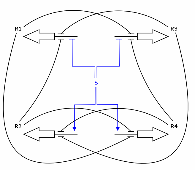
Recall the counter architecture:
We want to describe the concentrations of R1 - R4 over time given the input signal S. We will set up a deterministic model using ordinary differential equations (ODEs), as this approach is commonly used in modelling gene networks.
General approach
We have to formulate for each gene product an ODE describing its rate of change. This rate is comprised of a term characterizing the synthesis rate and one characterizing the degradation rate.
We assume that the degradation rate of a protein depends linearly on its concentration, i.e.
deg(p) = -k_deg*p
where k_deg is a degradation constant.
As for the synthesis rate we have to consider that gene expression is controlled by regulatory proteins, either
in an activating or a repressing manner.
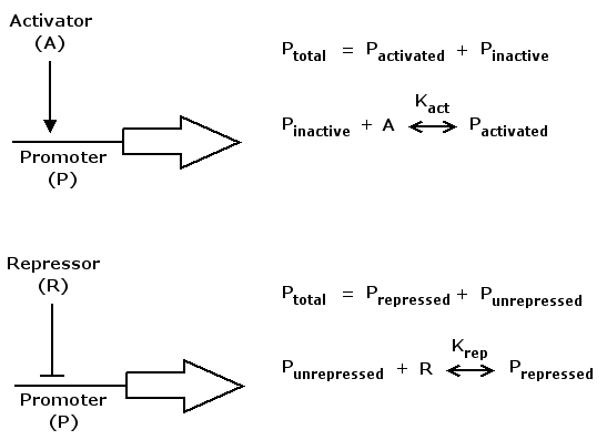
Mathematically, activation kann be formulated in the following way
act(A) = (K_act*A)^n / (1+(K_act*A)^n)
where A is a regulatory protein activating gene expression, K_act is a constant characterizing promoter-activator affinity (see figure above) and n describes the cooperativity of the activator. act(A) is in the range of [0 .. 1] and increases monotonically with increasing A.
Repression can be formulated accordingly
rep(R) = 1 / (1+(K_rep*R)^n)
where R is a regulatory protein repressing gene expression, K_rep and n are the equivalents of K_act and n in the activation case. rep(R) is in the range of [0 .. 1] and decreases monotonically with increasing R.
To get a synthesis rate we can multiply both act() and rep() with a kinetic constant k that describes the maximum synthesis rate. So on the one hand act() and rep() denote the synthesis rate relative to the maximum rate. On the other hand we can interpret them as probabilities. That is, the probability of any RNA polymerase molecule binding to the respective promoter and starting the protein synthesis process.
The total rate of change is then obtained by adding together the degradation and synthesis rates.
Application to the counter circuit
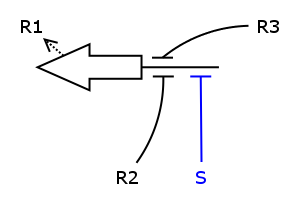
We now have all the building blocks we need to construct the ODEs for R1 - R4. Let's have a closer look at one of those Rs, say R1.
As one can see, the production of R1 depends on S, R2 and R3, i.e. S activates the production and R2/R3 repress it. We assume the individual repressors and activators affect the synthesis of R1 independently from each other, which means we can use the expressions for activation and repression that we have already formulated for each regulator separately. As we stated above the values of act() and rep() can be interpreted as probabilities. So what we need to model is the probability of three independent events coinciding. As we know from probability theory we obtain the desired probability by multiplying the individual event probabilities. Gluing everything together we get
dR1/dt = k_syn_R1 * act(S) * rep(R2) * rep(R3)  -  k_deg_R1 * R1
         \_________________ _________________/  \_______ _______/
                           V                            V
                    synthesis rate               degradation rate
Similarly we construct the other equations
 dR2/dt = k_syn_R2 * rep(S) * rep(R3) * rep(R4)  -  k_deg_R2 * R2
 dR3/dt = k_syn_R3 * act(S) * rep(R1) * rep(R4)  -  k_deg_R3 * R3
 dR4/dt = k_syn_R4 * rep(S) * rep(R1) * rep(R2)  -  k_deg_R4 * R4
Possible model improvements
Since the biological implementation of the circuit is split up into the Input Device and 4 overlapping NOR Devices, a more detailed/sophisticated model would probably give a better approximation to the actual circuit.
Matlab Code
Zipped Matlab Code
For those who want to try out the Matlab code, please use the zipped version and not the *.m files on the wiki (because those have been adapted to fit into the wiki and hence contain mistakes).
[http://www.tik.ee.ethz.ch/%7ebarkows/counter.zip Matlab gezippt]
Simulation for people who don't know how to handle Matlab
- If you don't have Matlab on your computer, install it (unfortunately, it's payware).
- Save all the *.m files (Matlab-files) from the zipped Matlab Code to your computer.
- Open Matlab.
- Set the 'Current Directory' path (above the Matlab terminal) to the folder where you stored the *.m files.
- In the file 'maincounter.m', set the parameters you want to simulate.
- In the Matlab terminal, type 'maincounter' in the command line.
- The computation takes about 2 seconds. Matlab then draws a plot where you can see the impact your chosen parameters have on the concentractions.
How does the simulation work?
maincounter.m
The main program is maincounter.m. First, the parameters are defined. Secondly, Matlab solves the differential equation (which are defined in ode_counter.m) using ode15s. Thirdly, a plot containing the input signal and all four concentrations is created. Last, Matlab calls the function jury.m which tells us whether the concentrations oscillates (which of course is what we want).
ode_counter.m
Here, the differential equations are defined. These are in words: The variation of a protein's concentration is equal to the product of activation and repression (because zincfingers act as roadblocks) minus a fixed part of the concentration itself (degradation).
act.m
Here, the equation we use for activation is defined.
rep.m
Here, the equation we use for reprimation is defined.
input_signal.m
The input signal is defined. You can choose between different input signals. The default input signal is a sinusoidal oscillation with 'breaks' (sections where the input remains zero between the sinusoidal peaks).
jury.m
Here, the function test_oscillation.m is called for every one of the four concentrations. jury.m returns one if any of the test_oscillation.m calls returned one (i.e. it suffices if one concentration is properly oscillating, because we can then choose that one to be the 'counting' concentration).
test_oscillation.m
Although the code looks quite complicating, what it does is pretty simple: It looks if the peaks (which of course have to occur with half the frequency of the input signal) are at least twice as big than the biggest point between the peaks (caused by noise).
What if I want to automatically test several sets of parameters?
You have set all parameters and done a simulation run. The result is negative (i.e. the concentrations don't oscillate correctly). You think you know which parameter you have to change to achieve a positive result, but you don't know how much you need to change it. There are two ways of finding that out:
- Change the parameter of interest by hand and do a simulation run. Look at the plot, and write down if that specific value works. Change the parameter again, do another simulation run, etc. If you want to test a large range of values (e.g. K from 1 to 1000 with stepsize 5), this approach is way too onerous (200 iterations). Instead, try the following:
- Use the function K_kd_iterate.m.
K_kd_iterate.m
Until now, only an iteration of K (zincfinger affinity) and kd (zincfinger degradation rate) has been implemented.
It works as follows: Create a vector with the values to be tested (of K and kd, respectively). Note that a higher K means a higher affinity (see the repression equation rep.m for details).
K_kd_iterate.m calls maincounter_iterate.m for every possible combination of K and kd. Be careful not to chose too large vectors. If you try 20 values for K and 20 values for kd, the computation takes a little more than ten (!) minutes.
maincounter_iterate.m
maincounter_iterate.m is the same as maincounter.m, only adapted to be used by K_kd_iterate.m (i.e. you can't set the parameters K and kd anymore).


